
https://tutorials.pytorch.kr/beginner/blitz/neural_networks_tutorial.html
신경망(Neural Networks)
신경망은 torch.nn 패키지를 사용하여 생성할 수 있습니다. 지금까지 autograd 를 살펴봤는데요, nn 은 모델을 정의하고 미분하는데 autograd 를 사용합니다. nn.Module 은 계층(layer)과 output 을 반환하는 for
tutorials.pytorch.kr
위의 글을 보면서, 내가 이해하기 쉽게 정리한 내용이다. 난 정리하면서 이해하는 편이라...처음 보는 사람들은 위의 글을 참고하는게 더 이해가 쉬울듯하다.

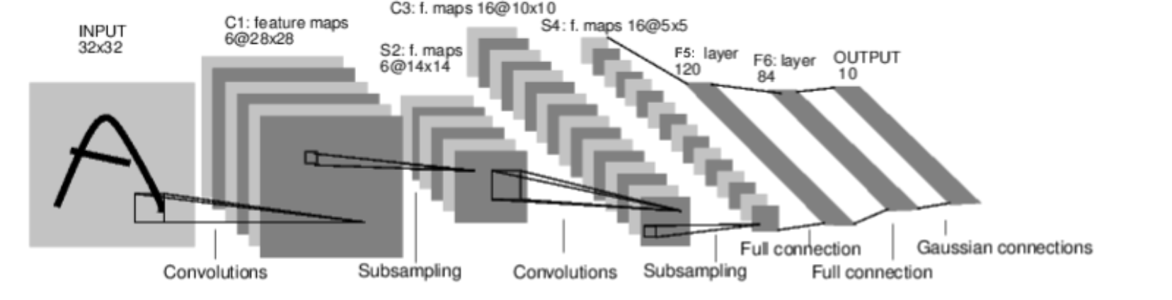
1. Neural Network 설계
설계해볼 Neural Network는 숫자 이미지를 분류하는 신경망 예제이다.
import torch
from torch.autograd import Variable
import torch.nn as nn
import torch.nn.functional as F


class Net(nn.Module):

    def __init__(self):
        super(Net, self).__init__()
        # 1개의 input channel, 6개의 output channels, 5x5 square convolution
        # 하나의 feature map size: (32-5+1) * (32-5+1) = 28 * 28
        self.conv1 = nn.Conv2d(1, 6, 5)

        # 6개의 input channel, 16개의 output channels, 5X5 square convolution
        # 하나의 feature map size: (16-5+1) * (16-5+1) = 10 * 10
        self.conv2 = nn.Conv2d(6, 16, 5)

        # an affine operation: y = Wx + b
        self.fc1 = nn.Linear(16 * 5 * 5, 120)
        self.fc2 = nn.Linear(120, 84)
        self.fc3 = nn.Linear(84, 10)

    def forward(self, x):
        # Max pooling over a (2, 2) window
        x = F.max_pool2d(F.relu(self.conv1(x)), (2, 2))
        # If the size is a square you can only specify a single number
        x = F.max_pool2d(F.relu(self.conv2(x)), 2)
        x = x.view(-1, self.num_flat_features(x))
        x = F.relu(self.fc1(x))
        x = F.relu(self.fc2(x))
        x = self.fc3(x)
        return x

    def num_flat_features(self, x):
        size = x.size()[1:]  # all dimensions except the batch dimension
        num_features = 1
        for s in size:
            num_features *= s
        return num_features


net = Net()
print(net)
위의 print 함수의 결과로 다음이 출력된다.
Net(
  (conv1): Conv2d(1, 6, kernel_size=(5, 5), stride=(1, 1))
  (conv2): Conv2d(6, 16, kernel_size=(5, 5), stride=(1, 1))
  (fc1): Linear(in_features=400, out_features=120, bias=True)
  (fc2): Linear(in_features=120, out_features=84, bias=True)
  (fc3): Linear(in_features=84, out_features=10, bias=True)
)
위와 같이 forward 함수만 정의하면 backward 함수는 autograd에 의해 자동으로 정의된다고 한다.
임의의 32X32 입력값을 network에 넣어보자.
input = torch.randn(1, 1, 32, 32)
out = net(input)
print(out)
결과는 다음과 같이 출력된다.
tensor([[ 0.0322,  0.0265,  0.0670,  0.0794,  0.0115, -0.0833,  0.0716,  0.1177,
         -0.1024, -0.1093]], grad_fn=<AddmmBackward0>)
2. 손실 함수 (Loss function)
loss function은 (output, target)을 한쌍으로 입력받아서, output이 target(정답)으로부터 얼마나 떨어져있는지 추정하는 값을 계산한다. nn 패키지엔 여러가지 손실 함수들이 존재하는데, 대표적인 손실함수로, output과 target간의 평균 제곱오차(mean-squared error)를 계산하는 nn.MSEloss가 있다.
output = net(input)
target = torch.randn(10)  # 예시를 위한 임의의 정답
target = target.view(1, -1)  # target을 출력과 같은 shape로 만듦
criterion = nn.MSELoss()

loss = criterion(output, target)
print(loss)
결과는 다음과 같이 출력된다.
tensor(0.7185, grad_fn=<MseLossBackward0>)
3. 역전파
error를 역전파해주기 위해서는 loss.backward()만 하면 된다. 역전파를 시키기 전에 모든 매개변수의 변화도 버퍼를 0으로 만드는 작업이 필요하다.
net.zero_grad()
loss.backward()
4. 가중치 weight 갱신
가중치 갱신 규칙은 다양하게 존재한다. SGD, Nesterov-SGD, Adam, RMSProp 등 다양한 규칙들이 있는데 이들은 모두 torch.optim이라는 패키지에 구현되어 있다. 다음과 같이 사용할 수 있다.
import torch.optim as optim

# Optimizer를 정의
optimizer = optim.SGD(net.parameters(), lr = 0.01)

# 학습과정(training loop는 다음과 같다)
optimizer.zero_grad()
output = net(input)
loss = criterion(output, target)
loss.backward()
optimizer.step() # 업데이트 진행
이렇게 pytorch를 사용하여 nerual network를 간단하게 정의하고 학습시키는 방법까지 알아보았다 ㅎㅎ
'연구 > PyTorch' 카테고리의 다른 글
| [PyTorch] Tensor 조작법 기본) indexing, view, squeeze, unsqueeze (0) | 2023.09.17 |
|---|---|
| PyTorch로 AutoEncoder 구현하기 (0) | 2023.08.16 |
| PyTorch DataLoader 사용하기 & epoch, batch, iteration 개념 (0) | 2023.08.03 |
| Pytorch에서 TensorBoard 사용하기 (0) | 2023.08.03 |
| Pytorch로 dataset 구성하기 (0) | 2023.07.27 |